How lead is calculated in War Thunder: ballistics, drift and flight time
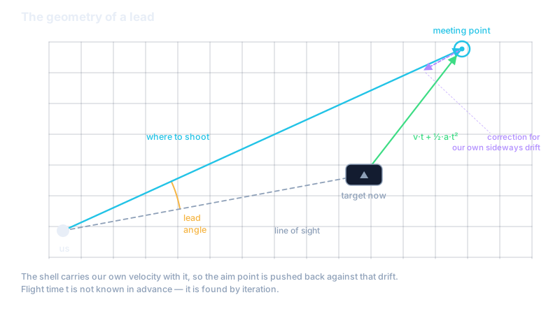
The lead marker in War Thunder looks simple: a circle ahead of the target, shoot there. Behind that circle sits a problem with no closed-form solution — it has to be solved numerically, several times per frame. Here is how.
The problem
Known: where the target is now, how fast and with what acceleration it is moving, where we are, how fast we are flying ourselves, and which shell is in the barrel. Wanted: the elevation and azimuth at which the shell and the target arrive at the same point.
The difficulty is that flight time depends on where you aim, and where you aim depends on flight time. That circle only opens up through iteration.
Air: density and drag
The shell is not flying in a vacuum. Air density falls with altitude, and deceleration depends on it directly. At the surface density is taken as 1.225 kg/m³ and computed from there as a polynomial in altitude — the model is cut off at 20 kilometres, above which there are no battles.
The speed of sound is derived the same way: a base of 288.16 metres per second corrected by a polynomial in altitude. It matters where the transonic transition does.
Density and the shell's own parameters give the drag coefficient:
k = −(ρ · π · 0.5 · r² · L) / m
where ρ is air density, r is half the calibre, L is shell length and m is its mass. The minus sign is not decorative: the coefficient is later multiplied by velocity, and the sign is what makes the result deceleration rather than thrust.
What the formula means in practice: a heavy shell of small calibre loses less speed. That is exactly why an APDS round keeps a flat trajectory where HE has already started to droop, and why the lead differs between them out of the same gun.
The trajectory: Runge–Kutta integration
The shell's acceleration at any instant:
dv/dt = k · |v| · v + g
Drag is proportional to the square of velocity — hence the |v| — and gravity adds a constant −9.81 m/s² downward. The equation is non-linear and has no analytic solution.
The path is stepped at 1/32 of a second with fourth-order Runge–Kutta: on each step acceleration is evaluated four times — at the start, twice in the middle and at the end — and the results are averaged 1:2:2:1. That is orders of magnitude more accurate than plain Euler at the same step size, which matters here because the error accumulates: over three kilometres, crude integration misses by metres.
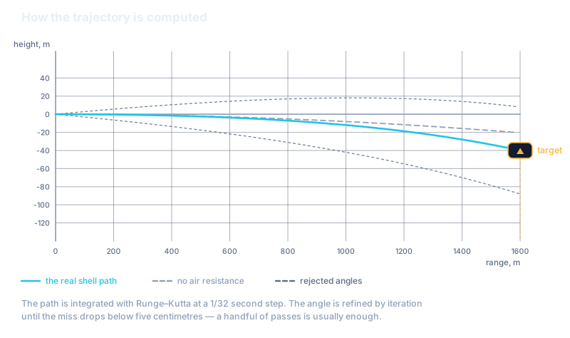
The simulation stops on one of three conditions: the shell has crossed the target's range, the shell has physically passed the target, or the flight time limit of 20 seconds has run out.
Refining the angle
The angle is found by iteration, always starting from the line of sight — the straight line from us to the target. Then, on each step:
- A full trajectory simulation runs at the current angle.
- Where the shell arrived at the target's range is measured.
- The angle is corrected by the difference between the arrival angle and the angle to the target.
Iteration stops once the miss is under five centimetres — noticeably finer than a hit requires, and well inside the gun's own dispersion. The cap is 100 iterations, though in practice a handful suffices.
Divergence is caught separately. If the miss grows five times running, the iteration stops. Under heavy drag the descent is not monotonic, so one or two worse steps are not enough to declare divergence — the threshold is five.
And there is a fallback: the best result across all iterations is kept. If five centimetres was never reached but the best miss is under 1% of the range and the angle has not wandered far from the line of sight, the solution is accepted anyway. A slightly less precise answer beats no answer and a target lost for a frame.
Your own velocity: why the linear correction is off by a kilometre
In an air fight we are moving too, and the shell carries our velocity with it. The along-track component simply adds to muzzle velocity. The cross-track component, though, pushes the shell sideways, and the aim point has to move against that drift.
This is where it is easy to go wrong. It feels natural to compute drift as "cross velocity × flight time". That is incorrect, and badly so: the shell decelerates, and the cross component decays exactly as the along-track one does — both obey the same equation with a shared |v| factor, so their ratio stays constant for the whole flight.
Which gives the correct estimate:
drift = v_cross · (ground range / initial horizontal speed)
The difference is not cosmetic. Checked against full three-dimensional integration, the linear estimate for a 20 mm cannon at 2.5 km overstated the drift by 1240 metres. The formula above matches the exact result.
Flight time: an equation with two roots
That leaves the circle to close. Write g(t) for the shell's flight time to the point where the target will be in t seconds. We want a t where g(t) = t — that is, a root of
f(t) = g(t) − t
For a receding air target g is convex and increasing, so f has two roots: a flat one around a second or two, and a lofted one somewhere near 15–18 seconds.
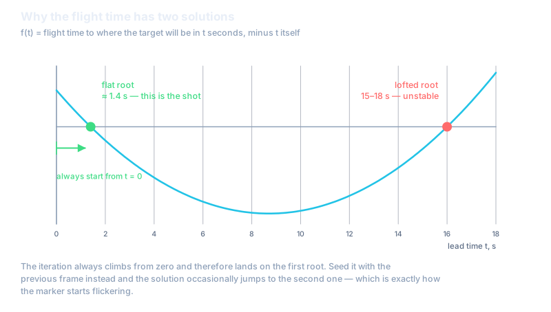
The first is the one we want. The second root is unstable: the derivative there exceeds one in magnitude, and an iteration started near it crawls away from it.
So the search always begins at t = 0, where f(0) = g(0) > 0, and climbs to the first root. On a convex function neither a fixed-point step nor a secant step overshoots it. Tolerance is 10 milliseconds of flight time: more than enough for aiming, and comfortably above floating-point noise.
If numerical noise does throw the estimate past the root, bisection takes over — the root is already bracketed, and inside that bracket it is unique.
Why the marker used to jump
The natural move is to seed the search with the previous frame's answer — the target has barely moved, after all. In practice that is precisely what broke the sight.
Let a manoeuvring target change the geometry and last frame's seed lands closer to the second root than the first. The iteration walks off to the lofted solution, the marker jumps halfway across the sky, then comes back. Starting from zero removes the dependence on the previous frame entirely: the solution is always the flat one, and always the same for the same situation.
What it buys you in a match
Accurate lead matters most where an error costs most: anti-air fire at a manoeuvring target, shooting on the move, long range at high tiers. At three kilometres the gap between "roughly there" and a computed meeting point is the gap between a hit and a tracer going past.
Lead modules, capture radius and aim modes are configured separately — see what is available in the War Thunder cheat description. How vehicles are drawn and coloured by visibility is covered in how the cheat draws vehicles in War Thunder.
The same problem looks different elsewhere: ballistics and sight zeroing in PUBG, the projectile speed table in Rust, aim smoothing in Apex Legends.